Video demonstrations
Click a video to play, or Explore in 3D to rotate, zoom and scrub through the flight.
Office
INDOOR 02Shopping mall
INDOOR 03Pisa
OUTDOOR 01Neuschwanstein
OUTDOOR 02Liberty
OUTDOOR 03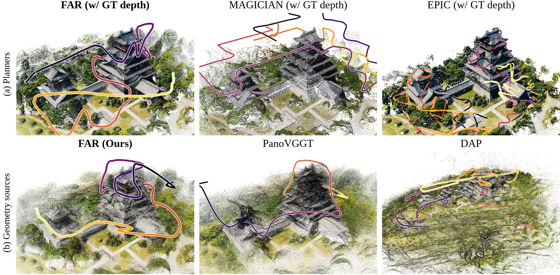
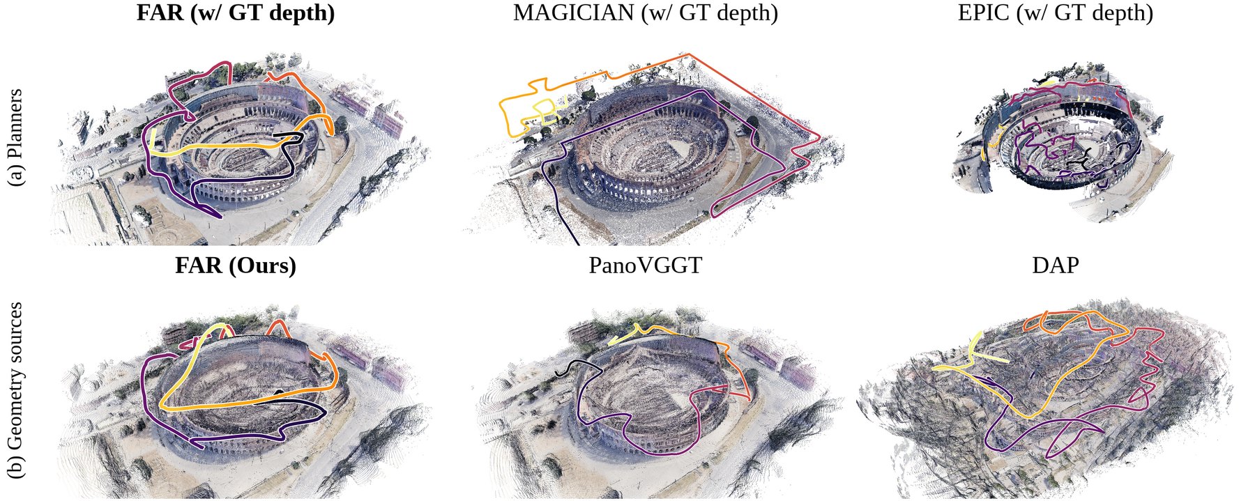
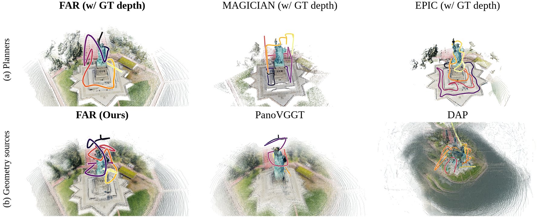
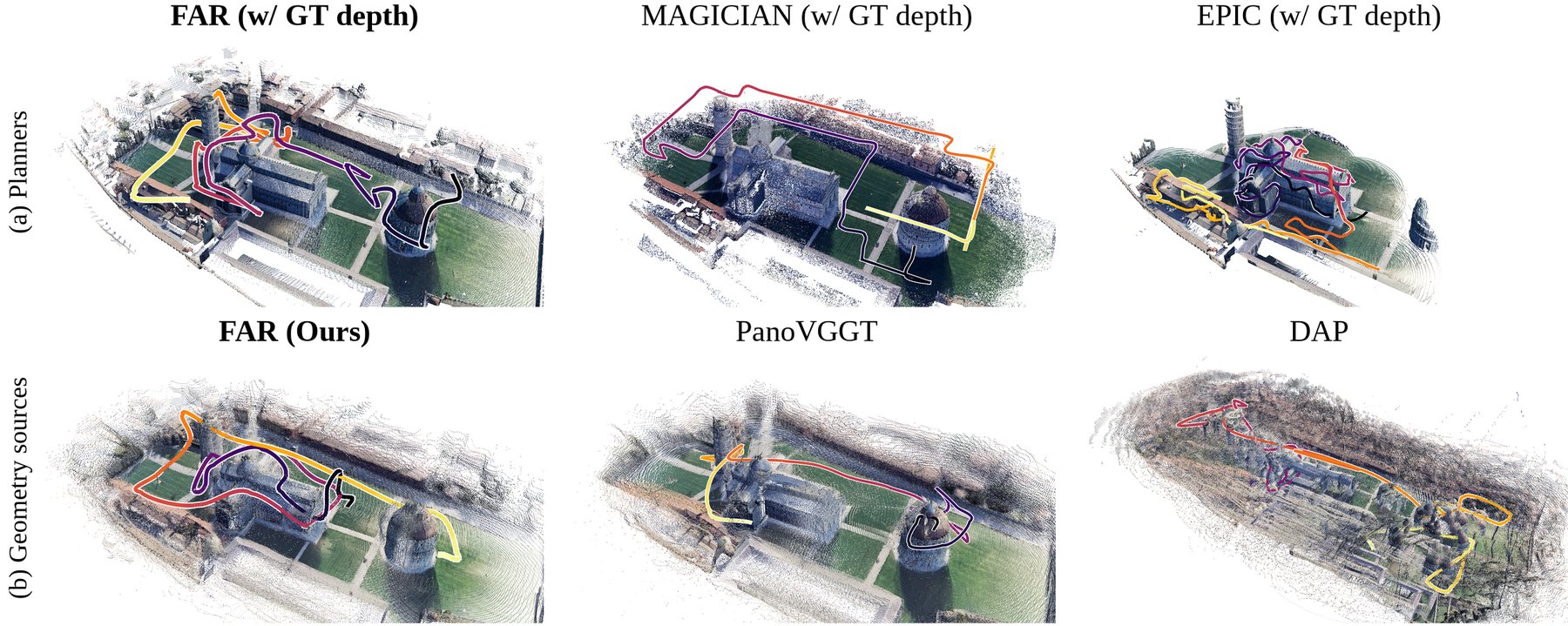
Shared reviewer questions
Reconstruction ablations
* qiHD Q1; eJ88 Q1
FAR combines panoramic depth prediction, metric alignment and persistent mapping to select the next capture position.
INPUTPanoramic RGB
+ metric poses
→+ metric poses
PERCEPTIONSRA depth
prediction
→prediction
GEOMETRYMetric alignment
+ persistent map
→+ persistent map
PLANNINGNext capture
position
position
FAR achieves the lowest AbsRel among the shown reconstruction ablations.
With the same planner, FAR achieves higher coverage and AUC than PanoVGGT using predicted depth.
| Method | Depth source | Coverage at ε = 1.0 m ↑ | AUC ↑ |
|---|---|---|---|
| FAR | GT depth (reference) | 85.6% | 0.663 |
| PanoVGGT | Predicted depth | 69.2% | 0.421 |
| FAR | Predicted depth | 83.3% | 0.634 |
Best results within each comparable group are shown in bold black text with an orange background. Ties are highlighted equally.
Same FAR planner. Only the two predicted depth rows are compared for highlighting; GT depth is a reference.
Comparison under matched sensing
* qiHD Q2; zcV1 Q1
With matched sensing, FAR achieves the highest coverage.
With matched sensing, FAR has the shortest flight path.
With the sensor fixed, FAR retains higher coverage and shorter paths.
| Sensor configuration | Method | Coverage at ε = 1.0 m ↑ | Path length (m) ↓ | AUC ↑ |
|---|---|---|---|---|
| Native (Table 1 in the main paper) | EPIC | 65.6% | 1807 | 0.377 |
| Native (Table 1 in the main paper) | MAGICIAN | 79.4% | 1400 | 0.500 |
| Native (Table 1 in the main paper) | FAR | 85.6% | 1111 | 0.663 |
| Omnidirectional, 50 m | EPIC | 67.4% | 1756 | 0.437 |
| Omnidirectional, 50 m | MAGICIAN | 80.5% | 1795 | 0.604 |
| Omnidirectional, 50 m | FAR | 85.2% | 1571 | 0.623 |
Best results within each comparable group are shown in bold black text with an orange background. Ties are highlighted equally.
Tables R1/R4 · GT depth, ε = 1.0 m. Native and matched sensor groups are compared separately. Added results are averaged over multiple start positions per scene.
Planning ablations
* zcV1 Q1; eJ88 Q4
Compared with FAR, removing Adaptive Initialization lowers final coverage; removing peak ratio termination lengthens the path with little additional coverage.
Adaptive Initialization adds 4.1 pp coverage; removing peak ratio termination adds only 0.4 pp but increases path length by 21%.
| Setting | Coverage at ε = 1.0 m ↑ | Path length (m) ↓ |
|---|---|---|
| FAR | 85.6% | 1111 |
| w/o Adaptive Initialization (one fixed parameter set for all scenes) | 81.5% | 888 |
| w/o termination based on the peak ratio | 86.0% | 1345 |
| MAGICIAN | 79.4% | 1400 |
| EPIC | 65.6% | 1807 |
Best results within each comparable group are shown in bold black text with an orange background. Ties are highlighted equally.
Tables R5/R13 · Native sensing, GT depth, ε = 1.0 m. Added results are averaged over multiple start positions per scene. Fixed settings use Colosseum’s adaptive values for all scenes. Removing peak ratio termination means η = 0.
Computational cost and decision rate
* qiHD Q3; zcV1 Q4
FAR has lower reported computational and memory costs than MAGICIAN and plans faster than EPIC.
| Method | Perception (ms) ↓ | Mapping (ms) ↓ | Planning (ms) ↓ | RAM (GB) ↓ | GPU memory (GB) ↓ |
|---|---|---|---|---|---|
| EPIC | — | 55 | 59 | 2.2 | 0 |
| MAGICIAN | 1282 | 175 | 3843 | 4.1 | 15.1 |
| FAR | 912 | 149 | 44 | 2.5 | 8.7 |
Best results within each comparable group are shown in bold black text with an orange background. Ties are highlighted equally.
R2/R8 · AMD EPYC 9T24, 32 vCPUs; RTX 5880 Ada, 48 GB. Latency: mean of per scene medians. Memory: mean of per run peaks.
VIEWPOINT DECISIONS0.78 Hz0.72–0.81 Hz across 11 scenes
Decision frequency, not total mission speed.
FAR achieves a viewpoint decision rate of 0.78 Hz.
| Metric | Median | P95 |
|---|---|---|
| Panorama rendering and readback (ms) | 42 | 72 |
| Perception per window (ms) | 912 | 1002 |
| Mapping (ms) | 149 | 221 |
| Planning per decision (ms) | 44 | 133 |
| Closed loop rate (Hz) | 0.78 | — |
Reviewer specific questions
qiHDCommon rendering pipeline+
Rendering quality with a common FastGS pipeline
* qiHD Q4
With FastGS fixed, FAR has higher PSNR and SSIM and lower LPIPS than MAGICIAN.
| Method | 3DGS training | Initial geometry | PSNR ↑ | SSIM ↑ | LPIPS ↓ |
|---|---|---|---|---|---|
| MAGICIAN | FastGS | GT depth | 13.14 | 0.397 | 0.447 |
| FAR (original paper)reference | SPaGS | Predicted depth | 15.94 | 0.452 | 0.429 |
| FAR (FastGS) | FastGS | Predicted depth | 15.29 | 0.434 | 0.443 |
Best results within each comparable group are shown in bold black text with an orange background. Ties are highlighted equally.
FastGS rows are compared; original SPaGS is reference only. Same ten ERP test positions per scene and matched FastGS training configuration. MAGICIAN: GT geometry; FAR: predicted geometry.
zcV1Training and pose inputs+
Training data and SRA ablations
* zcV1 Q2
With the same backbone and training data, SRA reduces AbsRel from 0.1914 to 0.1196.
| Model | Additional training data | AbsRel ↓ | RMSE (m) ↓ | δ₁.₂₅ ↑ |
|---|---|---|---|---|
| PanoVGGT | None | 0.1667 | 27.18 | 0.7684 |
| PanoVGGT | Ours (FAR26 + Holo360D) | 0.1274 | 24.36 | 0.8473 |
| VGGT-Ω w/o SRA | Ours (FAR26 + Holo360D) | 0.1914 | 31.46 | 0.6821 |
| VGGT-Ω + SRA (ours) | Ours (FAR26 + Holo360D) | 0.1196 | 23.29 | 0.8647 |
Best results within each comparable group are shown in bold black text with an orange background. Ties are highlighted equally.
All rows use the same alignment. PanoVGGT’s additional training uses the same data, steps and mixture as FAR; w/o SRA updates only the depth head. Macarons++ evaluation scenes are absent from training.
Comparison with MapAnything
* zcV1 Q3
Within each alignment group, FAR outperforms MapAnything on all three reported metrics.
| Method | Use of poses | AbsRel ↓ | δ₁.₂₅ ↑ | RMSE (m) ↓ |
|---|---|---|---|---|
| MapAnything (cubemap) | Within the network | 0.3555 | 0.3481 | 55.8 |
| Ours w/o alignment | Within the network | 0.2073 | 0.5872 | 37.72 |
| MapAnything (cubemap) + alignment | Within the network and for alignment | 0.2189 | 0.6385 | 36.54 |
| Ours (SRA + alignment) | Within the network and for alignment | 0.1196 | 0.8647 | 23.29 |
Best results within each comparable group are shown in bold black text with an orange background. Ties are highlighted equally.
Without alignment, FAR outperforms MapAnything on all test scenes. Both receive the same metric poses. Compare within each alignment group; MapAnything uses cubemap to ERP adaptation.
eJ88Robustness, detail and disclosure+
Component adaptations
* eJ88 Q1
FAR adapts ray encoding, persistent mapping and planning to panoramic active reconstruction.
| Prior component | FAR adaptation |
|---|---|
| UCPE | ERP seam handling, pole frame fallback, metric camera offsets. |
| AMB3R | A global voxel map that persists across windows. |
| FUEL | Routing retained; Adaptive Initialization and peak ratio termination added. |
Parameter sensitivity
* eJ88 Q2
Across all 25 settings, coverage changes range from −4.4 to +1.6 pp; the minimum is 81.2%.
| α / default α | η = 0.03 | η = 0.05 | η = 0.07 | η = 0.10 | η = 0.15 |
|---|---|---|---|---|---|
| ×0.5 | −1.0 | −1.2 | −1.4 | −1.5 | −1.9 |
| ×0.7 | +1.6 | +1.6 | +0.9 | +0.7 | 0.0 |
| ×1 | +0.5 | +0.3 | 0 (default) | −0.3 | −1.5 |
| ×1.4 | −1.6 | −1.8 | −2.0 | −2.3 | −2.9 |
| ×2 | −3.6 | −3.6 | −3.7 | −3.8 | −4.4 |
At η = 0.07, finer voxel settings increase path length by 33–54%.
| α / default α | η = 0.03 | η = 0.05 | η = 0.07 | η = 0.10 | η = 0.15 |
|---|---|---|---|---|---|
| ×0.5 | 1.76 | 1.63 | 1.54 | 1.41 | 1.25 |
| ×0.7 | 1.51 | 1.44 | 1.33 | 1.25 | 1.14 |
| ×1 | 1.19 | 1.09 | 1.00 (default) | 0.94 | 0.87 |
| ×1.4 | 0.88 | 0.86 | 0.83 | 0.79 | 0.76 |
| ×2 | 0.67 | 0.67 | 0.66 | 0.65 | 0.63 |
GT depth, 11 scenes, multiple start positions per scene. Default: α = 0.0273, η = 0.07, coverage 85.6%. Coverage uses ε = 1.0 m; path values are ratios to the default. Shading shows values; the outline marks the default.
Local detail at matched flight budgets
* eJ88 Q3
Adaptive voxels achieve the highest detail AUC in both scenes under the same path budget.
| Scene | Voxel size (m) | Coverage at ε = 0.5 m | AUC at ε = 0.5 m under the same path budget | Path length (m) |
|---|---|---|---|---|
| Colosseum | 2.25 | 64.6% | 0.512 | 2477 (+53%) |
| Colosseum | 3.15 | 63.3% | 0.518 | 2103 (+30%) |
| Colosseum | 4.5 (adaptive) | 62.0% | 0.533 | 1615 |
| Dunnottar | 2.22 | 98.8% | 0.742 | 1883 (+34%) |
| Dunnottar | 3.11 | 98.0% | 0.783 | 1470 (+5%) |
| Dunnottar | 4.45 (adaptive) | 98.4% | 0.813 | 1401 |
Best results within each comparable group are shown in bold black text with an orange background. Ties are highlighted equally.
ε = 0.5 m; compare within each scene. AUC uses the same path budget.
Closed loop comparisons
* eJ88 Q4
Initialization and termination ablations are provided; the persistent versus per window closed loop comparison is not included.
| Comparison | Available evidence |
|---|---|
| Fixed vs adaptive parameters | R5/R13 and the planning curve above. |
| With vs without peak ratio termination | R5/R13 and the planning curve above. |
| Persistent vs per window refinement | Closed loop coverage/path comparison not included. |
Parameter settings and task boundary
* eJ88 Q5; eJ88 Q6
All 11 scenes share the same parameters, and the task boundary closely encloses the target structure.
| Item | Reported setting |
|---|---|
| α default | 0.0273; selected for mapping and planning efficiency. |
| η default | 0.07; coverage saturation criterion. |
| Across scenes | One shared setting across all 11 scenes. |
| Task boundary B | Official Macarons++ evaluation box, closely enclosing the target. |
Figure 1 provenance and AI disclosure
* eJ88 AI Disclosure Concern
The central “Omnidirectional View” panel in Figure 1 combines three elements: a 3D scene generated with OpenAI’s ChatGPT Image based on one of our existing scenes, a photograph of our actual UAV, and a panoramic sphere in the upper left created from visual materials in PowerPoint. This composition illustrates omnidirectional acquisition, with the generated scene designed to enhance the sense of depth and convey this concept more clearly. All other result images in the paper were produced by our experiments. We apologize for omitting this use of image generation from the AI Use Statement; we will revise the statement in the main manuscript and update the Figure 1 caption to disclose the generated scene and explain the composition.